直线拟合原理
给出多个点,然后根据这些点拟合出一条直线,这个最常见的算法是多约束方程的最小二乘拟合,如下图所示:

但是当这些点当中有一个或者几个离群点(outlier)时候,最小二乘拟合出来的直线就直接翻车成这样了:

原因是最小二乘无法在估算拟合的时候剔除或者降低离群点的影响,于是一个聪明的家伙出现了,提出了基于权重的最小二乘拟合估算方法,这样就避免了翻车。根据高斯分布,离群点权重应该尽可能的小,这样就可以降低它的影响,OpenCV中的直线拟合就是就权重最小二乘完成的,在生成权重时候OpenCV支持几种不同的距离计算方法,分别如下:

其中DIST_L2是最原始的最小二乘,最容易翻车的一种拟合方式,虽然速度快点。然后用基于权重的最小二乘估算拟合结果如下:

函数与实现源码分析
OpenCV中直线拟合函数支持上述六种距离计算方式,函数与参数解释如下:
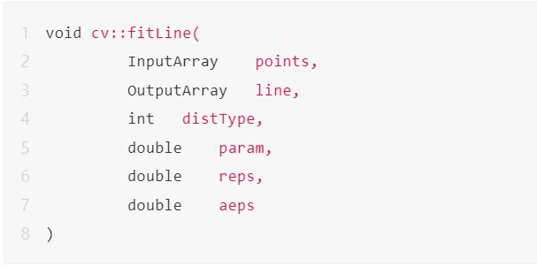
points是输入点集合
line是输出的拟合参数,支持2D与3D
distType是选择距离计算方式
param 是某些距离计算时生成权重需要的参数
reps 是前后两次原点到直线的距离差值,可以看成拟合精度高低
aeps是前后两次角度差值,表示的是拟合精度
六种权重的计算更新实现如下:
staticvoidweightL1(float*d,intcount,float*w) { inti; for(i=0;i< count; i++ ) { double t = fabs( (double) d[i] ); w[i] = (float)(1. / MAX(t, eps)); } } static void weightL12( float *d, int count, float *w ) { int i; for( i = 0; i < count; i++ ) { w[i] = 1.0f / (float) std::sqrt( 1 + (double) (d[i] * d[i] * 0.5) ); } } static void weightHuber( float *d, int count, float *w, float _c ) { int i; const float c = _c <= 0 ? 1.345f : _c; for( i = 0; i < count; i++ ) { if( d[i] < c ) w[i] = 1.0f; else w[i] = c/d[i]; } } static void weightFair( float *d, int count, float *w, float _c ) { int i; const float c = _c == 0 ? 1 / 1.3998f : 1 / _c; for( i = 0; i < count; i++ ) { w[i] = 1 / (1 + d[i] * c); } } static void weightWelsch( float *d, int count, float *w, float _c ) { int i; const float c = _c == 0 ? 1 / 2.9846f : 1 / _c; for( i = 0; i < count; i++ ) { w[i] = (float) std::exp( -d[i] * d[i] * c * c ); } }拟合计算的代码实现:
staticvoidfitLine2D_wods(constPoint2f*points,intcount,float*weights,float*line) { CV_Assert(count>0); doublex=0,y=0,x2=0,y2=0,xy=0,w=0; doubledx2,dy2,dxy; inti; floatt; //Calculatingtheaverageofxandy… if(weights==0) { for(i=0;i< count; i += 1 ) { x += points[i].x; y += points[i].y; x2 += points[i].x * points[i].x; y2 += points[i].y * points[i].y; xy += points[i].x * points[i].y; } w = (float) count; } else { for( i = 0; i < count; i += 1 ) { x += weights[i] * points[i].x; y += weights[i] * points[i].y; x2 += weights[i] * points[i].x * points[i].x; y2 += weights[i] * points[i].y * points[i].y; xy += weights[i] * points[i].x * points[i].y; w += weights[i]; } } x /= w; y /= w; x2 /= w; y2 /= w; xy /= w; dx2 = x2 – x * x; dy2 = y2 – y * y; dxy = xy – x * y; t = (float) atan2( 2 * dxy, dx2 – dy2 ) / 2; line[0] = (float) cos( t ); line[1] = (float) sin( t ); line[2] = (float) x; line[3] = (float) y; }案例:直线拟合
有如下的原图:

通过OpenCV的距离变换,骨架提取,然后再直线拟合,使用DIST_L1得到的结果如下:

审核编辑:刘清
免责声明:文章内容来自互联网,本站不对其真实性负责,也不承担任何法律责任,如有侵权等情况,请与本站联系删除。
转载请注明出处:一文简析OpenCV中的直线拟合方法-opencv绘制直方图 https://www.yhzz.com.cn/a/8118.html