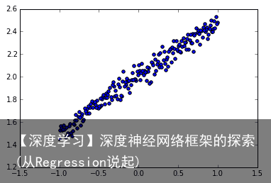
神经网络可以用来模拟回归问题 (regression),例如给下面一组数据,用一条线来对数据进行拟合,并可以预测新输入 x 的输出值。  导入模块并创建数据 models.Sequential,用来一层一层一层的去建立神经层; layers.Dense 意思是这个神经层是全连接层。
 建立模型 然后用 Sequential 建立 model, 再用 model.add 添加神经层,添加的是 Dense 全连接神经层。
参数有两个,一个是输入数据和输出数据的维度,本代码的例子中 x 和 y 是一维的。
如果需要添加下一个神经层的时候,不用再定义输入的纬度,因为它默认就把前一层的输出作为当前层的输入。在这个例子里,只需要一层就够了。
model = Sequential() model.add(Dense(output_dim=1, input_dim=1))
激活模型 接下来要激活神经网络,上一步只是定义模型。
参数中,误差函数用的是 mse 均方误差;优化器用的是 sgd 随机梯度下降法。
choose loss function and optimizing methodmodel.compile(loss=mse, optimizer=sgd) 以上三行就构建好了一个神经网络,它比 Tensorflow 要少了很多代码,很简单。
可视化结果 最后可以画出预测结果,与测试集的值进行对比。
plotting the predictionY_pred = model.predict(X_test) plt.scatter(X_test, Y_test) plt.plot(X_test, Y_pred) plt.show() 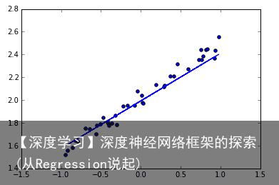
近几年最火的深度学习框架是什么?毫无疑问,TensorFlow 高票当选。同时Caffe、PyTorch、MXNet、CNTK用得也非常多。这些框架虽各有优势,但都具有一些普遍特征,据Gokula Krishnan Santhanam总结,大部分深度学习框架都包含以下五个核心组件:
(1)张量(Tensor) 的数据结构。 (2)基于张量的各种操作。 (3) (Computation Graph) (4) (Automatic Differentiation) (5) BLAS cuBLAS. cuDNN 4 tiRE.其中,张量(Tensor)可以理解为任意维度的数组一-比 如一维数组被称作向量(Vector) ,三维的被称作矩阵(Matrix) ,这些都属于张量。有了张量,就有对应的基本操作,如取某行某列的值、张量乘以常数等。运用拓展包其实就相当于使用底层计算软件加速运算。我们今天重点介绍的就是计算图模型和自动微分两部分。首先谈谈如何实现自动求导,然后用最简单的方法实现这两部分。
3 基于反向传播算法的自动求导首先看正向传播。给定函数e= (a+ b)(b+1),当a=2、b=1时,进行正向传播,其实就是小学乘法,即将a=2、 b=1带入,e=(a+b)(b+ 1)=3×2=6。反向传播过程就麻烦一-些了.我们暂日可以将这个式子直接运用求导法则进行求导。
自动微分(Automatic Differentiation,简称AD)也称自动求导,算法能够计算可导函数在某点处的导数值的计算,是反向传播算法的一般化。自动微分要解决的核心问题是计算复杂函数,通常是多层复合函数在某一点处的导数,梯度,以及Hessian矩阵值。它对用户屏蔽了繁琐的求导细节和过程。目前知名的深度学习开源库均提供了自动微分的功能,包括TensorFlow、pytorch等。
对于编程计算目标函数的导数值,目前有4种方法:手动微分,数值微分,符号微分,以及自动微分,在接下来会分别进行介绍。
自动微分在深度学习库中的地位
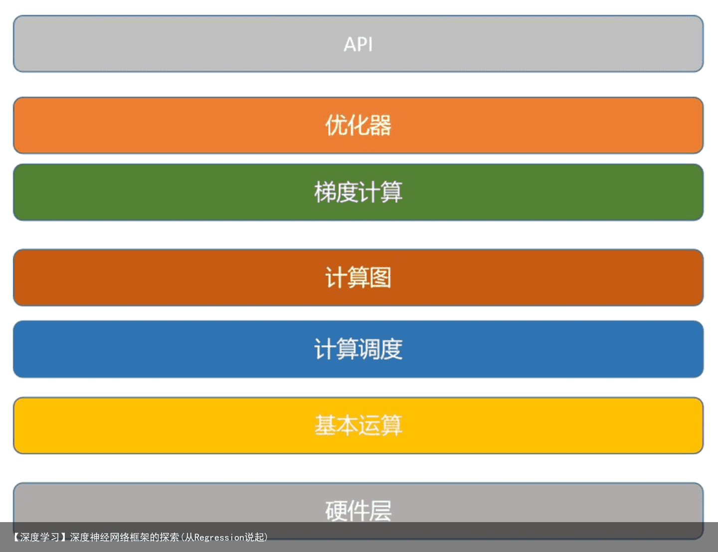
自动微分技术在深度学习库中处于重要地位,是整个训练算法的核心组件之一。一个典型的深度学习库架构如下图所示。在这里忽略了网络通信,本地IO等模块。
 梯度计算一般使用本文所讲述的自动微分技术,计算出梯度值给优化器使用,用于训练阶段。如果使用标准的梯度下降法进行迭代,在第k次迭代时的计算公式为

可以理解为看你和真实值差多少而已,然后反向传播,不断调整。
4 简单深度神经网络框架实现4.1 数据结构
class Node(object): “”” Base class for nodes in the network. Arguments: `inbound_nodes`: A list of nodes with edges into this node. “”” def __init__(self, inbound_nodes=[]): “”” Nodes constructor (runs when the object is instantiated). Sets properties that all nodes need. “”” # A list of nodes with edges into this node. self.inbound_nodes = inbound_nodes # The eventual value of this node. Set by running # the forward() method. self.value = None # A list of nodes that this node outputs to. self.outbound_nodes = [] # New property! Keys are the inputs to this node and # their values are the partials of this node with # respect to that input. self.gradients = {} # Sets this node as an outbound node for all of # this nodes inputs. for node in inbound_nodes: node.outbound_nodes.append(self) def forward(self): “”” Every node that uses this class as a base class will need to define its own `forward` method. “”” raise NotImplementedError def backward(self): “”” Every node that uses this class as a base class will need to define its own `backward` method. “”” raise NotImplementedError class Input(Node): “”” A generic input into the network. “”” def __init__(self): Node.__init__(self) def forward(self): pass def backward(self): self.gradients = {self: 0} for n in self.outbound_nodes: self.gradients[self] += n.gradients[self] class Linear(Node): “”” Represents a node that performs a linear transform. “”” def __init__(self, X, W, b): Node.__init__(self, [X, W, b]) def forward(self): “”” Performs the math behind a linear transform. “”” X = self.inbound_nodes[0].value W = self.inbound_nodes[1].value b = self.inbound_nodes[2].value self.value = np.dot(X, W) + b def backward(self): “”” Calculates the gradient based on the output values. “”” self.gradients = {n: np.zeros_like(n.value) for n in self.inbound_nodes} for n in self.outbound_nodes: grad_cost = n.gradients[self] self.gradients[self.inbound_nodes[0]] += np.dot(grad_cost, self.inbound_nodes[1].value.T) self.gradients[self.inbound_nodes[1]] += np.dot(self.inbound_nodes[0].value.T, grad_cost) self.gradients[self.inbound_nodes[2]] += np.sum(grad_cost, axis=0, keepdims=False) class Sigmoid(Node): “”” Represents a node that performs the sigmoid activation function. “”” def __init__(self, node): Node.__init__(self, [node]) def _sigmoid(self, x): “”” This method is separate from `forward` because it will be used with `backward` as well. `x`: A numpy array-like object. “”” return 1. / (1. + np.exp(-x)) def forward(self): “”” Perform the sigmoid function and set the value. “”” input_value = self.inbound_nodes[0].value self.value = self._sigmoid(input_value) def backward(self): “”” Calculates the gradient using the derivative of the sigmoid function. “”” self.gradients = {n: np.zeros_like(n.value) for n in self.inbound_nodes} for n in self.outbound_nodes: grad_cost = n.gradients[self] sigmoid = self.value self.gradients[self.inbound_nodes[0]] += sigmoid * (1 – sigmoid) * grad_cost class MSE(Node): def __init__(self, y, a): “”” The mean squared error cost function. Should be used as the last node for a network. “”” Node.__init__(self, [y, a]) def forward(self): “”” Calculates the mean squared error. “”” y = self.inbound_nodes[0].value.reshape(-1, 1) a = self.inbound_nodes[1].value.reshape(-1, 1) self.m = self.inbound_nodes[0].value.shape[0] self.diff = y – a self.value = np.mean(self.diff**2) def backward(self): “”” Calculates the gradient of the cost. “”” self.gradients[self.inbound_nodes[0]] = (2 / self.m) * self.diff self.gradients[self.inbound_nodes[1]] = (-2 / self.m) * self.diff4.2 计算图组件
源深度学习库Tensorflow通过计算图(Computational Graph)表述计算流程。学过数据结构的同学都不会对图的概念陌生。Tensorflow中的每一个数据都是计算图上的一个节点,节点之间的边描述了数据之间的计算即流向关系。下面是一个典型的计算图。
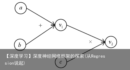 该图所表示的运算为

其中节点 v1,v2为表示中间结果或最终结果的变量。在后面的讲述中,将会以计算图作为工具。
# python def topological_sort(feed_dict): “”” Sort the nodes in topological order using Kahns Algorithm. `feed_dict`: A dictionary where the key is a `Input` Node and the value is the respective value feed to that Node. Returns a list of sorted nodes. “”” input_nodes = [n for n in feed_dict.keys()] G = {} nodes = [n for n in input_nodes] while len(nodes) > 0: n = nodes.pop(0) if n not in G: G[n] = {in: set(), out: set()} for m in n.outbound_nodes: if m not in G: G[m] = {in: set(), out: set()} G[n][out].add(m) G[m][in].add(n) nodes.append(m) L = [] S = set(input_nodes) while len(S) > 0: n = S.pop() if isinstance(n, Input): n.value = feed_dict[n] L.append(n) for m in n.outbound_nodes: G[n][out].remove(m) G[m][in].remove(n) if len(G[m][in]) == 0: S.add(m) return L4.3 训练模型(部分代码)
一个优化例子: 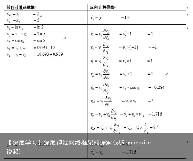 再看代码:
再看代码:
免责声明:文章内容来自互联网,本站不对其真实性负责,也不承担任何法律责任,如有侵权等情况,请与本站联系删除。
转载请注明出处:【深度学习】深度神经网络框架的探索(从Regression说起) https://www.yhzz.com.cn/a/12605.html