【深度学习】EfficientNetV2分析总结和flops的开源库
1 EfficientNetV1中存在的问题 2 EfficientNetV2中做出的贡献 3 NAS 搜索 4 EfficientNetV2网络框架 4.1 EfficientNetV2-M的详细参数 4.2 EfficientNetV2-L的详细参数 5 EfficientNetV2与其他模型训练时间对比 6 代码 7 FLOPs总结 8 计算flops的开源库 1 EfficientNetV1中存在的问题
作者系统性的研究了EfficientNet的训练过程,并总结出了三个问题:
训练图像的尺寸很大时,训练速度非常慢。 这确实是个槽点,在之前使用EfficientNet时发现当使用到B3(img_size=300)- B7(img_size=600)时基本训练不动,而且非常吃显存。通过下表可以看到,在Tesla V100上当训练的图像尺寸为380×380时,batch_size=24还能跑起来,当训练的图像尺寸为512×512时,batch_size=24时就报OOM(显存不够)了。针对这个问题一个比较好想到的办法就是降低训练图像的尺寸,之前也有一些文章这么干过。降低训练图像的尺寸不仅能够加快训练速度,还能使用更大的batch_size. 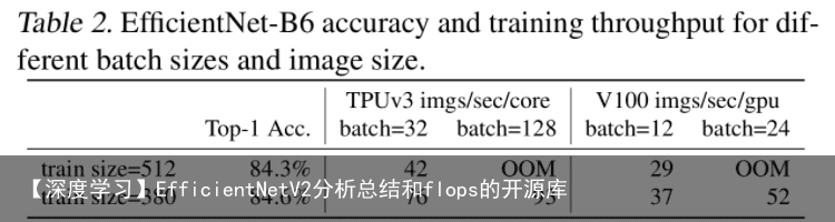
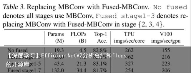
 在网络浅层中使用Depthwise convolutions速度会很慢。 虽然Depthwise convolutions结构相比普通卷积拥有更少的参数以及更小的FLOPs,但通常无法充分利用现有的一些加速器(虽然理论上计算量很小,但实际使用起来并没有想象中那么快)。在近些年的研究中,有人提出了Fused-MBConv结构去更好的利用移动端或服务端的加速器。Fused-MBConv结构也非常简单,即将原来的MBConv结构(之前在将EfficientNetv1时有详细讲过)主分支中的expansion conv1x1和depthwise conv3x3替换成一个普通的conv3x3,如图2所示。作者也在EfficientNet-B4上做了一些测试,发现将浅层MBConv结构替换成Fused-MBConv结构能够明显提升训练速度,如表3所示,将stage2,3,4都替换成Fused-MBConv结构后,在Tesla V100上从每秒训练155张图片提升到216张。但如果将所有stage都替换成Fused-MBConv结构会明显增加参数数量以及FLOPs,训练速度也会降低。所以作者使用NAS技术去搜索MBConv和Fused-MBConv的最佳组合。
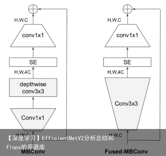
2 EfficientNetV2中做出的贡献
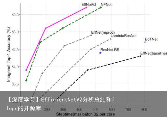
在之前的一些研究中,大家主要关注的是准确率以及参数数量(注意,参数数量少并不代表推理速度更快)。但在近些年的研究中,大家开始关注网络的训练速度以及推理速度(可能是准确率刷不动了)。但他们提升训练速度通常是以增加参数数量作为代价的。而这篇文章是同时关注训练速度以及参数数量的。
这篇文章做出的三个贡献:
引入新的网络(EfficientNetV2),该网络在训练速度以及参数数量上都优于先前的一些网络。 提出了改进的渐进学习方法,该方法会根据训练图像的尺寸动态调节正则方法(例如dropout、data augmentation和mixup)。通过实验展示了该方法不仅能够提升训练速度,同时还能提升准确率。 通过实验与先前的一些网络相比,训练速度提升11倍,参数数量减少为1/6.8 。
3 NAS 搜索
这部分自己看论文最好。
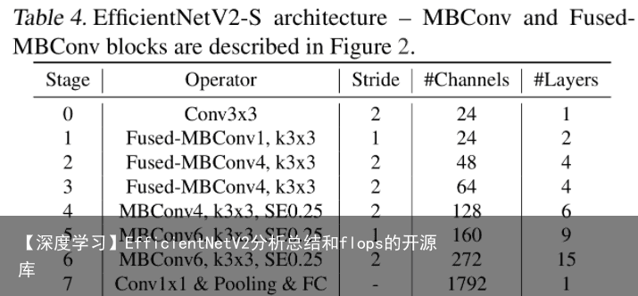
4 EfficientNetV2网络框架
4.1 EfficientNetV2-M的详细参数
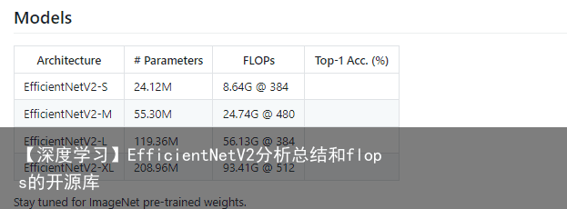
EfficientNetV2-M的配置是在baseline的基础上采用了width倍率因子1.6, depth倍率因子2.2得到的(这两个倍率因子是EfficientNetV1-B5中采用的)。
4.2 EfficientNetV2-L的详细参数
EfficientNetV2-L的配置是在baseline的基础上采用了width倍率因子2.0, depth倍率因子3.1得到的(这两个倍率因子是EfficientNetV1-B7中采用的)。
5 EfficientNetV2与其他模型训练时间对比
6 代码
import torch
import torch.nn as nn
import math
__all__ = [effnetv2_s, effnetv2_m, effnetv2_l, effnetv2_xl]
def _make_divisible(v, divisor, min_value=None):
“””
This function is taken from the original tf repo.
It ensures that all layers have a channel number that is divisible by 8
It can be seen here:
https://github.com/tensorflow/models/blob/master/research/slim/nets/mobilenet/mobilenet.py
:param v:
:param divisor:
:param min_value:
:return:
“””
if min_value is None:
min_value = divisor
new_v = max(min_value, int(v + divisor / 2) // divisor * divisor)
# Make sure that round down does not go down by more than 10%.
if new_v < 0.9 * v:
new_v += divisor
return new_v
# SiLU (Swish) activation function
if hasattr(nn, SiLU):
SiLU = nn.SiLU
else:
# For compatibility with old PyTorch versions
class SiLU(nn.Module):
def forward(self, x):
return x * torch.sigmoid(x)
class SELayer(nn.Module):
def __init__(self, inp, oup, reduction=4):
super(SELayer, self).__init__()
self.avg_pool = nn.AdaptiveAvgPool2d(1)
self.fc = nn.Sequential(
nn.Linear(oup, _make_divisible(inp // reduction, 8)),
SiLU(),
nn.Linear(_make_divisible(inp // reduction, 8), oup),
nn.Sigmoid()
)
def forward(self, x):
b, c, _, _ = x.size()
y = self.avg_pool(x).view(b, c)
y = self.fc(y).view(b, c, 1, 1)
return x * y
def conv_3x3_bn(inp, oup, stride):
return nn.Sequential(
nn.Conv2d(inp, oup, 3, stride, 1, bias=False),
nn.BatchNorm2d(oup),
SiLU()
)
def conv_1x1_bn(inp, oup):
return nn.Sequential(
nn.Conv2d(inp, oup, 1, 1, 0, bias=False),
nn.BatchNorm2d(oup),
SiLU()
)
class MBConv(nn.Module):
def __init__(self, inp, oup, stride, expand_ratio, use_se):
super(MBConv, self).__init__()
assert stride in [1, 2]
hidden_dim = round(inp * expand_ratio)
self.identity = stride == 1 and inp == oup
if use_se:
self.conv = nn.Sequential(
# pw
nn.Conv2d(inp, hidden_dim, 1, 1, 0, bias=False),
nn.BatchNorm2d(hidden_dim),
SiLU(),
# dw
nn.Conv2d(hidden_dim, hidden_dim, 3, stride, 1, groups=hidden_dim, bias=False),
nn.BatchNorm2d(hidden_dim),
SiLU(),
SELayer(inp, hidden_dim),
# pw-linear
nn.Conv2d(hidden_dim, oup, 1, 1, 0, bias=False),
nn.BatchNorm2d(oup),
)
else:
self.conv = nn.Sequential(
# fused
nn.Conv2d(inp, hidden_dim, 3, stride, 1, bias=False),
nn.BatchNorm2d(hidden_dim),
SiLU(),
# pw-linear
nn.Conv2d(hidden_dim, oup, 1, 1, 0, bias=False),
nn.BatchNorm2d(oup),
)
def forward(self, x):
if self.identity:
return x + self.conv(x)
else:
return self.conv(x)
class EffNetV2(nn.Module):
def __init__(self, cfgs, num_classes=1000, width_mult=1.):
super(EffNetV2, self).__init__()
self.cfgs = cfgs
# building first layer
input_channel = _make_divisible(24 * width_mult, 8)
layers = [conv_3x3_bn(3, input_channel, 2)]
# building inverted residual blocks
block = MBConv
for t, c, n, s, use_se in self.cfgs:
output_channel = _make_divisible(c * width_mult, 8)
for i in range(n):
layers.append(block(input_channel, output_channel, s if i == 0 else 1, t, use_se))
input_channel = output_channel
self.features = nn.Sequential(*layers)
# building last several layers
output_channel = _make_divisible(1792 * width_mult, 8) if width_mult > 1.0 else 1792
self.conv = conv_1x1_bn(input_channel, output_channel)
self.avgpool = nn.AdaptiveAvgPool2d((1, 1))
self.classifier = nn.Linear(output_channel, num_classes)
self._initialize_weights()
def forward(self, x):
x = self.features(x)
x = self.conv(x)
x = self.avgpool(x)
x = x.view(x.size(0), -1)
x = self.classifier(x)
return x
def _initialize_weights(self):
for m in self.modules():
if isinstance(m, nn.Conv2d):
n = m.kernel_size[0] * m.kernel_size[1] * m.out_channels
m.weight.data.normal_(0, math.sqrt(2. / n))
if m.bias is not None:
m.bias.data.zero_()
elif isinstance(m, nn.BatchNorm2d):
m.weight.data.fill_(1)
m.bias.data.zero_()
elif isinstance(m, nn.Linear):
m.weight.data.normal_(0, 0.001)
m.bias.data.zero_()
def effnetv2_s(**kwargs):
“””
Constructs a EfficientNetV2-S model
“””
cfgs = [
# t, c, n, s, SE
[1, 24, 2, 1, 0],
[4, 48, 4, 2, 0],
[4, 64, 4, 2, 0],
[4, 128, 6, 2, 1],
[6, 160, 9, 1, 1],
[6, 272, 15, 2, 1],
]
return EffNetV2(cfgs, **kwargs)
def effnetv2_m(**kwargs):
“””
Constructs a EfficientNetV2-M model
“””
cfgs = [
# t, c, n, s, SE
[1, 24, 3, 1, 0],
[4, 48, 5, 2, 0],
[4, 80, 5, 2, 0],
[4, 160, 7, 2, 1],
[6, 176, 14, 1, 1],
[6, 304, 18, 2, 1],
[6, 512, 5, 1, 1],
]
return EffNetV2(cfgs, **kwargs)
def effnetv2_l(**kwargs):
“””
Constructs a EfficientNetV2-L model
“””
cfgs = [
# t, c, n, s, SE
[1, 32, 4, 1, 0],
[4, 64, 7, 2, 0],
[4, 96, 7, 2, 0],
[4, 192, 10, 2, 1],
[6, 224, 19, 1, 1],
[6, 384, 25, 2, 1],
[6, 640, 7, 1, 1],
]
return EffNetV2(cfgs, **kwargs)
def effnetv2_xl(**kwargs):
“””
Constructs a EfficientNetV2-XL model
“””
cfgs = [
# t, c, n, s, SE
[1, 32, 4, 1, 0],
[4, 64, 8, 2, 0],
[4, 96, 8, 2, 0],
[4, 192, 16, 2, 1],
[6, 256, 24, 1, 1],
[6, 512, 32, 2, 1],
[6, 640, 8, 1, 1],
]
return EffNetV2(cfgs, **kwargs)
<
7 FLOPs总结
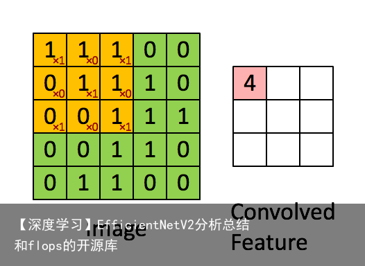
 我们知道,通常我们去评价一个模型时,首先看的应该是它的精确度,当你精确度不行的时候,你和别人说我的模型预测的多么多么的快,部署的时候占的内存多么多么的小,都是白搭。但当你模型达到一定的精确度之后,就需要更进一步的评价指标来评价你模型:1)前向传播时所需的计算力,它反应了对硬件如GPU性能要求的高低;2)参数个数,它反应所占内存大小。为什么要加上这两个指标呢?因为这事关你模型算法的落地。比如你要在手机和汽车上部署深度学习模型,对模型大小和计算力就有严格要求。模型参数想必大家都知道是什么怎么算了,而前向传播时所需的计算力可能还会带有一点点疑问。所以这里总计一下前向传播时所需的计算力。它正是由FLOPs体现,那么FLOPs该怎么计算呢? 我们知道,在一个模型进行前向传播的时候,会进行卷积、池化、BatchNorm、Relu、Upsample等操作。这些操作的进行都会有其对应的计算力消耗产生,其中,卷积所对应的计算力消耗是所占比重最高的。所以,我们这里主要讲一下卷积操作所对应的计算力。
我们以下图为例进行讲解:
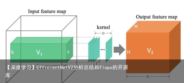 先说结论:卷积层 计算力消耗 等于上图中两个立方体 (绿色和橙色) 体积的乘积。即flops =

8 计算flops的开源库
https://github.com/sovrasov/flops-counter.pytorch