【深度学习】基于Pytorch的softmax回归问题辨析和应用(二)

我们可以发现(通过深度学习框架的高级API能够使实现
)
线性(回归变得更加容易)。同样地,通过深度学习框架的高级API也能更方便地实现分类模型。让我们继续使用Fashion-MNIST数据集,并保持批量大小为256. import torch from torch import nn from d2l import torch as d2l batch_size = 256 train_iter, test_iter = d2l.load_data_fashion_mnist(batch_size)
1.1 初始化模型参数
在 Sequential 中添加一个带有10个输出的全连接层。同样,在这里,Sequential 并不是必要的,但我们可能会形成这种习惯。因为在实现深度模型时,Sequential将无处不在。我们仍然以均值0和标准差0.01随机初始化权重。
# PyTorch不会隐式地调整输入的形状。因此, # 我们在线性层前定义了展平层(flatten),来调整网络输入的形状 net = nn.Sequential(nn.Flatten(), nn.Linear(784, 10)) def init_weights(m): if type(m) == nn.Linear: nn.init.normal_(m.weight, std=0.01) net.apply(init_weights);1.2 Softmax的实现
回想一下,softmax函数 $\hat y_j = \frac{\exp(o_j)}{\sum_k \exp(o_k)}$,其中$\hat y_j$是预测的概率分布。$o_j$是未归一化的预测$\mathbf{o}$的第$j$个元素。如果$o_k$中的一些数值非常大,那么 $\exp(o_k)$ 可能大于数据类型容许的最大数字(即 上溢(overflow))。这将使分母或分子变为inf(无穷大),我们最后遇到的是0、inf 或 nan(不是数字)的 $\hat y_j$。在这些情况下,我们不能得到一个明确定义的交叉熵的返回值。
解决这个问题的一个技巧是,在继续softmax计算之前,先从所有$o_k$中减去$\max(o_k)$。你可以证明每个 $o_k$ 按常数进行的移动不会改变softmax的返回值。在减法和归一化步骤之后,可能有些 $o_j$ 具有较大的负值。由于精度受限, $\exp(o_j)$ 将有接近零的值,即 下溢(underflow)。这些值可能会四舍五入为零,使 $\hat y_j$ 为零,并且使得 $\log(\hat y_j)$ 的值为 -inf。反向传播几步后,我们可能会发现自己面对一屏幕可怕的nan结果。
尽管我们要计算指数函数,但我们最终在计算交叉熵损失时会取它们的对数。
通过将softmax和交叉熵结合在一起,可以避免反向传播过程中可能会困扰我们的数值稳定性问题。如下面的等式所示,我们避免计算$\exp(o_j)$,而可以直接使用$o_j$。因为$\log(\exp(\cdot))$被抵消了。$$
\begin{aligned}
\log{(\hat y_j)} & = \log\left( \frac{\exp(o_j)}{\sum_k \exp(o_k)}\right) \
& = \log{(\exp(o_j))}-\log{\left( \sum_k \exp(o_k) \right)} \
& = o_j -\log{\left( \sum_k \exp(o_k) \right)}.
\end{aligned}
$$我们也希望保留传统的softmax函数,以备我们需要评估通过模型输出的概率。
但是,我们没有将softmax概率传递到损失函数中, loss = nn.CrossEntropyLoss()1.3 优化器
trainer = torch.optim.SGD(net.parameters(), lr=0.1)1.4 训练
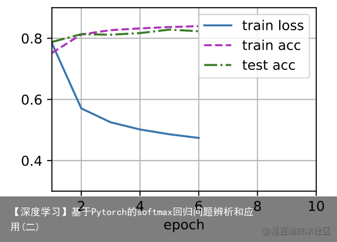
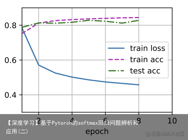
接下来我们实现一个训练函数,它会在train_iter 访问到的训练数据集上训练一个模型net。该训练函数将会运行多个迭代周期(由num_epochs指定)。在每个迭代周期结束时,利用 test_iter 访问到的测试数据集对模型进行评估。我们将利用 Animator 类来可视化训练进度。
def train_epoch_ch3(net, train_iter, loss, updater): #@save “””训练模型一个迭代周期(定义见第3章)。””” # 训练损失总和、训练准确度总和、样本数 metric = Accumulator(3) if isinstance(updater, gluon.Trainer): updater = updater.step for X, y in train_iter: # 计算梯度并更新参数 with autograd.record(): y_hat = net(X) l = loss(y_hat, y) l.backward() updater(X.shape[0]) metric.add(float(l.sum()), accuracy(y_hat, y), y.size) # 返回训练损失和训练准确率 return metric[0] / metric[2], metric[1] / metric[2]使用SGD优化器更新模型参数:
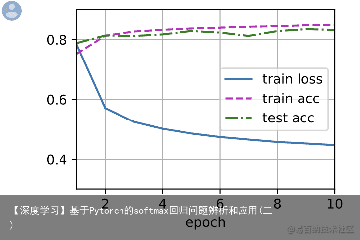
lr = 0.1 def updater(batch_size): return d2l.sgd([W, b], lr, batch_size) def train_ch3(net, train_iter, test_iter, loss, num_epochs, updater): #@save “””训练模型(定义见第3章)。””” animator = Animator(xlabel=epoch, xlim=[1, num_epochs], ylim=[0.3, 0.9], legend=[train loss, train acc, test acc]) for epoch in range(num_epochs): train_metrics = train_epoch_ch3(net, train_iter, loss, updater) test_acc = evaluate_accuracy(net, test_iter) animator.add(epoch + 1, train_metrics + (test_acc,)) train_loss, train_acc = train_metrics assert train_loss < 0.5, train_loss assert train_acc <= 1 and train_acc > 0.7, train_acc assert test_acc <= 1 and test_acc > 0.7, test_acc num_epochs = 10 d2l.train_ch3(net, train_iter, test_iter, loss, num_epochs, trainer)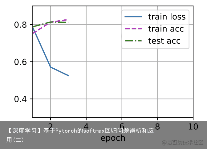
为什么谈论这个问题呢?是因为我在工作的过程中遇到了语义分割预测输出特征图个数为16,也就是所谓的16分类问题。
因为每个通道的像素的值的大小代表了像素属于该通道的类的大小,为了在一张图上用不同的颜色显示出来,我不得不学习了torch.nn.Softmax的使用。
首先看一个简答的例子,倘若输出为(3, 4, 4),也就是3张4×4的特征图。
import torch img = torch.rand((3,4,4)) print(img)输出为:
tensor([[[0.0413, 0.8728, 0.8926, 0.0693], [0.4072, 0.0302, 0.9248, 0.6676], [0.4699, 0.9197, 0.3333, 0.4809], [0.3877, 0.7673, 0.6132, 0.5203]], [[0.4940, 0.7996, 0.5513, 0.8016], [0.1157, 0.8323, 0.9944, 0.2127], [0.3055, 0.4343, 0.8123, 0.3184], [0.8246, 0.6731, 0.3229, 0.1730]], [[0.0661, 0.1905, 0.4490, 0.7484], [0.4013, 0.1468, 0.2145, 0.8838], [0.0083, 0.5029, 0.0141, 0.8998], [0.8673, 0.2308, 0.8808, 0.0532]]])我们可以看到共三张特征图,每张特征图上对应的值越大,说明属于该特征图对应类的概率越大。
import torch.nn as nn sogtmax = nn.Softmax(dim=0) img = sogtmax(img) print(img) tensor([[[0.2780, 0.4107, 0.4251, 0.1979], [0.3648, 0.2297, 0.3901, 0.3477], [0.4035, 0.4396, 0.2993, 0.2967], [0.2402, 0.4008, 0.3273, 0.4285]], [[0.4371, 0.3817, 0.3022, 0.4117], [0.2726, 0.5122, 0.4182, 0.2206], [0.3423, 0.2706, 0.4832, 0.2522], [0.3718, 0.3648, 0.2449, 0.3028]], [[0.2849, 0.2076, 0.2728, 0.3904], [0.3627, 0.2581, 0.1917, 0.4317], [0.2543, 0.2898, 0.2175, 0.4511], [0.3880, 0.2344, 0.4278, 0.2686]]])可以看到,上面的代码对每张特征图对应位置的像素值进行Softmax函数处理, 图中标红位置加和=1,同理,标蓝位置加和=1。
我们看到Softmax函数会对原特征图每个像素的值在对应维度(这里dim=0,也就是第一维)上进行计算,将其处理到0~1之间,并且大小固定不变。
print(torch.max(img,0))输出为:
torch.return_types.max( values=tensor([[0.4371, 0.4107, 0.4251, 0.4117], [0.3648, 0.5122, 0.4182, 0.4317], [0.4035, 0.4396, 0.4832, 0.4511], [0.3880, 0.4008, 0.4278, 0.4285]]), indices=tensor([[1, 0, 0, 1], [0, 1, 1, 2], [0, 0, 1, 2], [2, 0, 2, 0]]))可以看到这里3x4x4变成了1x4x4,而且对应位置上的值为像素对应每个通道上的最大值,并且indices是对应的分类。
清楚理解了上面的流程,那么我们就容易处理了。
看具体案例,这里输出output的大小为:16x416x416.
output = torch.tensor(output) sm = nn.Softmax(dim=0) output = sm(output) mask = torch.max(output,0).indices.numpy() # 因为要转化为RGB彩色图,所以增加一维 rgb_img = np.zeros((output.shape[1], output.shape[2], 3)) for i in range(len(mask)): for j in range(len(mask[0])): if mask[i][j] == 0: rgb_img[i][j][0] = 255 rgb_img[i][j][1] = 255 rgb_img[i][j][2] = 255 if mask[i][j] == 1: rgb_img[i][j][0] = 255 rgb_img[i][j][1] = 180 rgb_img[i][j][2] = 0 if mask[i][j] == 2: rgb_img[i][j][0] = 255 rgb_img[i][j][1] = 180 rgb_img[i][j][2] = 180 if mask[i][j] == 3: rgb_img[i][j][0] = 255 rgb_img[i][j][1] = 180 rgb_img[i][j][2] = 255 if mask[i][j] == 4: rgb_img[i][j][0] = 255 rgb_img[i][j][1] = 255 rgb_img[i][j][2] = 180 if mask[i][j] == 5: rgb_img[i][j][0] = 255 rgb_img[i][j][1] = 255 rgb_img[i][j][2] = 0 if mask[i][j] == 6: rgb_img[i][j][0] = 255 rgb_img[i][j][1] = 0 rgb_img[i][j][2] = 180 if mask[i][j] == 7: rgb_img[i][j][0] = 255 rgb_img[i][j][1] = 0 rgb_img[i][j][2] = 255 if mask[i][j] == 8: rgb_img[i][j][0] = 255 rgb_img[i][j][1] = 0 rgb_img[i][j][2] = 0 if mask[i][j] == 9: rgb_img[i][j][0] = 180 rgb_img[i][j][1] = 0 rgb_img[i][j][2] = 0 if mask[i][j] == 10: rgb_img[i][j][0] = 180 rgb_img[i][j][1] = 255 rgb_img[i][j][2] = 255 if mask[i][j] == 11: rgb_img[i][j][0] = 180 rgb_img[i][j][1] = 0 rgb_img[i][j][2] = 180 if mask[i][j] == 12: rgb_img[i][j][0] = 180 rgb_img[i][j][1] = 0 rgb_img[i][j][2] = 255 if mask[i][j] == 13: rgb_img[i][j][0] = 180 rgb_img[i][j][1] = 255 rgb_img[i][j][2] = 180 if mask[i][j] == 14: rgb_img[i][j][0] = 0 rgb_img[i][j][1] = 180 rgb_img[i][j][2] = 255 if mask[i][j] == 15: rgb_img[i][j][0] = 0 rgb_img[i][j][1] = 0 rgb_img[i][j][2] = 0 cv2.imwrite(output.jpg, rgb_img)
免责声明:文章内容来自互联网,本站不对其真实性负责,也不承担任何法律责任,如有侵权等情况,请与本站联系删除。
转载请注明出处:【深度学习】基于Pytorch的softmax回归问题辨析和应用(二) https://www.yhzz.com.cn/a/11753.html